Introduction

Machine learning techniques, owing to their accuracy and precision, are being increasingly employed for decision making in a variety of scenarios. From stock purchases to marketing campaigns, organizations base their decisions on the insights obtained from data via machine learning techniques. This article demonstrates how machine learning automates the decision-making process of evaluating a car's condition.  You will see how to develop a machine learning model which predicts if a car is in an unacceptable, acceptable, good or very good condition, based on different characteristics of the car.  

Prerequisites

1. It is assumed that the readers have intermediate knowledge of the Python programming language since the code samples are in Python.
2. The code has been tested with Google Colaboratory.  However, you can run it on your local machines as well, provided you have installed Python 3.6.

Step 1: Problem Statement & Dataset

The task is to predict whether a car is in an unacceptable, acceptable, good or very good condition based on car characteristics such as the price of the car, maintenance cost, safety features, luggage space, seating capacity,  and the number of doors.

The dataset we will be using to build our model can be freely downloaded from this kaggle link.  The dataset is in CSV format. In case you are using a cloud platform to develop the model, you will need to upload the CSV file to the corresponding cloud platform.

Step 2: Importing Libraries and Loading the Dataset

The following script imports the libraries required to execute the scripts in this article:

‍

import pandas as pd
import numpy as np
from sklearn.metrics import classification_report, confusion_matrix, accuracy_score

import matplotlib.pyplot as plt
%matplotlib inline

import seaborn as sns
sns.set(style="darkgrid")

‍

If you open the CSV file for the dataset, you will see that it doesn't contain headers for data columns. The details of the headers for the dataset is available at this link.  If you look at the "Attribute Information"  heading at the link, you can see the details of the headers that correspond to different attributes of the cars.

There are 6 attributes in total:

1. buying:  which corresponds to the price of the car. There are four possible values for this attribute:  vhigh, high, med and low.
2. maint: which stands for the maintenance cost. It can also have the same four possible values as for the buying attribute.
3. doors: corresponds to the number of doors of a car. The possible values are 2, 3, 4, 5more.
4. persons: refers to the seating capacity of a car. The possible values are 2, 4 or more.
5. lug_boot: contains information about the luggage compartment, and can have small, med, and big as the possible values.
6. safety: corresponds to the safety rating of the car. The possible values are low, med, and high.
7. class: refers to the manual evaluation of the car's condition. A car can be in an unacceptable condition, acceptable condition, good condition, and very good condition. The shorthand notations for the values are unacc, acc, good, and vgood. The class attribute is renamed as condition for the sake of readability.

The task is to predict the value for the seventh attributes, given the values for the first six attributes.

The following script loads the dataset:

colnames=['buying', 'maint', 'doors', 'persons', 'lug_boot', 'safety','condition']
car_data = pd.read_csv(r'E:\Datasets\car_prediction.csv', names=colnames, header=None)

Let's first see how our dataset looks like.

car_data.head()

Output:

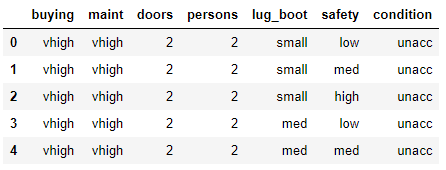
You can see the seven attributes in the dataset.  Let's now print the unique values for all the columns in our dataset.

for col in car_data:
   print("--")
   print(col)
   print (car_data[col].unique())

Output:

--
buying
['vhigh' 'high' 'med' 'low']
--
maint
['vhigh' 'high' 'med' 'low']
--
doors
['2' '3' '4' '5more']
--
persons
['2' '4' 'more']
--
lug_boot
['small' 'med' 'big']
--
safety
['low' 'med' 'high']
--
condition
['unacc' 'acc' 'vgood' 'good']

Step 3: Exploratory Data Analysis

Before training the model, it is always a good idea to perform some exploratory data analysis on the data.

Let's visualize the relationship between the output class i.e. condition and some of the other attributes in the dataset.

Firstly, we increase the default plot size with the following script:

plot_size = plt.rcParams["figure.figsize"]
plot_size [0] = 8
plot_size [1] = 6
plt.rcParams["figure.figsize"] = plot_size

The following script generates a pie plot that shows the class distribution for the condition column.  

car_data.condition.value_counts().plot(kind='pie', autopct='%1.0f%%', colors = ['skyblue', 'orange', 'pink', 'lightgreen'], explode = (0.05, 0.05, 0.05,0.05))

Output:

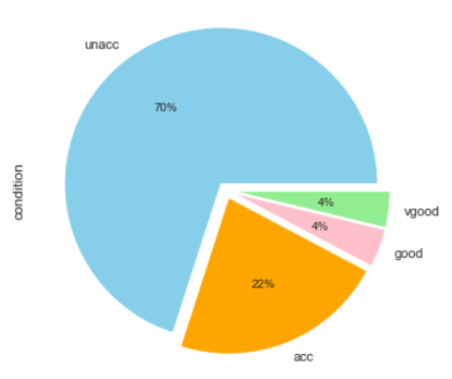
You can see that 70% of the cars have unacceptable conditions while 22% of the cars are in acceptable conditions. The ratio of cars with good and very good conditions is very low. 

Let's now see the relationship between the condition and buying attributes:

(car_data
.groupby(['condition', 'buying'])
.size()
.unstack()
.plot.bar()
)

Output:

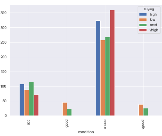
The output shows that cars with acceptable and unacceptable conditions belong to all price ranges. However, cars with good and very good conditions are either medium or low price cars. The possible reason for this distribution is that expensive cars might have better conditions than less expensive cars, however, the conditions of the expensive cars may not justify their price tags. Hence, with respect to their price, the condition has been rated as either acceptable or not acceptable, and not good or very good.

Next, let's plot the relationship between the conditions and doors attributes.

(car_data
.groupby(['condition', 'doors'])
.size()
.unstack()
.plot.bar()
)

Output:

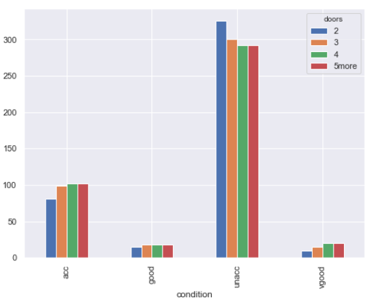
You can see that the distribution of cars with respect to the number of doors across various car condition types is approximately the same. Therefore, doors is not a very good attribute for decision making regarding a car's condition.

Finally, we will plot the relationship between condition and safety attributes.

(car_data
.groupby(['condition', 'safety'])
.size()
.unstack()
.plot.bar()
)

Output:

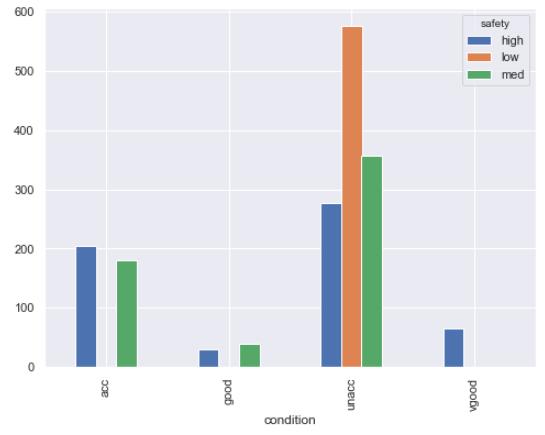
The output shows that none of the cars with low safety have been rated as being in acceptable, good or very good condition. All the cars with low safety features have been rated as having unacceptable conditions. Therefore, it can be assumed that safety is a very good feature for decision making regarding a car's condition.  In the same way, we can study the relationships between the remaining attributes in the dataset.

Step 4: Data Preprocessing

The basic purpose of exploratory data analysis is to see which are the most important features for decision making since a large number of features can really slow down the model training and can also negatively affect the performance of the algorithms. Exploratory data analysis and feature selection is a mandatory step in case you have large datasets.  However, since we have only 6 features to base our decision on, we will retain all of the features in the dataset and will apply pre-processing to all of them.

All the features in our dataset are categorical, i.e. they contain categorical values. Features that contain both numerical and categorical values, for instance,   doors and person are also treated as categorical features. However, machine learning algorithms work only with numbers. Therefore, we need to convert the categorical features in our dataset to their numerical counterparts. To do so, one-hot encoding can be used. In one hot encoding, for each value in a categorical column, a new column is created. The integer 1 is added to one of the newly generated columns that correspond to the actual value.

Let's first remove all the features or attributes from the car_data dataset, except `condition` since the condition is what we have to predict.  

temp_data =  car_data.drop(['buying', 'maint', 'doors', 'persons', 'lug_boot', 'safety'] , axis=1)

Next, we need to create one-hot encoded columns for the attributes that we dropped.

buying = pd.get_dummies(car_data.buying, prefix = 'buying')
maint = pd.get_dummies(car_data.maint, prefix = 'maint')

doors = pd.get_dummies(car_data.doors, prefix = 'doors')
persons = pd.get_dummies(car_data.persons, prefix = 'persons')

lug_boot = pd.get_dummies(car_data.lug_boot, prefix = 'lug_boot')
safety = pd.get_dummies(car_data.safety, prefix = 'safety')

Now, if you print the `buying` dataframe, you should see the following output:

buying.head()

Output:

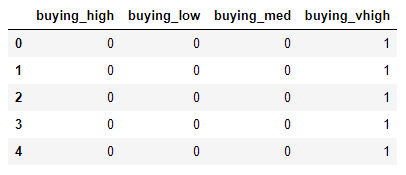
You can see that for each value in the original `buying` column, a new column has been generated.

Next, we need to concatenate the one-hot encoded columns for all the attributes to create the final dataset.

car_data = pd.concat([buying, maint, doors, persons, lug_boot, safety, temp_data] , axis=1)

Step 5: Training the Model

In this step, we will train our machine learning model on the data.  We will use the Random Forest algorithm to train our model. However, before that, we need to divide the dataset into training and test set. The model is trained on the training data and model performance is evaluated on the test data.

The following script divides the data into training and test sets:

X = car_data.loc[:, car_data.columns != 'condition'].values
y = car_data[['condition']]

from sklearn.model_selection import train_test_split
X_train, X_test, y_train, y_test = train_test_split(X, y, test_size=0.2, random_state=42)

Finally, the following script trains the model on the test set:

from sklearn.ensemble import RandomForestClassifier

model= RandomForestClassifier(n_estimators=20, random_state=0)
model.fit(X_train, y_train)
y_pred = model.predict(X_test)

Step 6: Evaluating Model Performance

Confusion matrix, accuracy, precision, and recall are the performance metrics used to evaluate the performance of a classification model such as the one we developed in this article. Look at the following script:

print(classification_report(y_test,y_pred))
print("\nConfusion Matrix:")
print(confusion_matrix(y_test,y_pred))

print("\nAccuracy:")
print(accuracy_score(y_test, y_pred))

Output:

  precision    recall  f1-score   support

        acc       0.95      0.88      0.91        83
       good       0.62      0.73      0.67        11
      unacc       0.98      1.00      0.99       235
      vgood       0.88      0.82      0.85        17

  micro avg       0.95      0.95      0.95       346
  macro avg       0.85      0.86      0.85       346
weighted avg       0.96      0.95      0.95       346


Confusion Matrix:
[[ 73   5   5   0]
[  1   8   0   2]
[  0   0 235   0]
[  3   0   0  14]]

Accuracy:
0.953757225433526

Our model achieves an accuracy of 95.37% which is pretty impressive.  

Conclusion

Car condition evaluation is one of the many decision-making problems that can be solved via machine learning techniques. This article explains how to automate the process of predicting the condition of any car based on several attributes such as price, safety, maintenance cost, etc. The article also explains how to perform exploratory data analysis for studying feature importance.